Hierarchy of Protocols
Quick Delete/Rarrange/Add/Save/Rename Scans
Adjusting Scan Parameters
Copy Slice Prescription
Other Interface 'Gotchas'
Scanner Interface Focus vs. Operator Mental Focus
Reformat Scan DICOMs to Different Plane
Export Data to YYMMDDHHII Directory on Linux Server (sni05)
User-defined Diffusion Directions
Siemens SMS (multiband) Product Sequence 'Gotchas'
Scanner Pulse and Bimanual Response Boxes, Outside Response Box
Video Connections
Setting Up the Front Projector (Hanging Screen)
Setting Up the Front Projector (Close-Up/Direct View)
Setting Up the Rear Projector
Projector Image 'Flips' for Front and Rear Projection
Visual Angle of Image
Kineticor-Compatible Mirror
OptoAcoustics Headphones/Mic Operation
20-channel Somatosensory Air Puffer Operation
Logging Siemens Physiological Data (pulse oximeter, respiration)
Shimming: Force new shim, Check shim applied, Manual shim
The Isocenter
Save/Export/Modify/Import Protocols
In-house cortical surface mapping software: csurf, mapper
How to Power Cycle the Helium Pump
A Selected Scan Won't Run
Scans only load/initiate when they are in the first non-grey position within the queue list. To reposition the desired scan and allow it to run (e.g., in case you decide to jump out of order and run a scan that is located at the middle or end of your protocol), left-click and drag the scan to the current top of the queue.
Note that if you have already selected the "Play" button to initiate the measurement/scan before click-dragging it into the correct position, the scanning sequence will immediately begin when properly positioned in the queue.
The easiest way to avoid problems like this is to start with a "Program" (set of protocols) that only contains a localizer (e.g., Marty -> Ex -> 32ch -> justloc). Then click on the "Program Card" icon (third icon up from bottom on far right), navigate to your intended Program, and simply click-drag individual scans out of there into the lower left queue to run them, one at a time. You can also click-drag the current scan to copy the slice prescription for another functional run.
This makes it much less likely for you to get mentally 'out of synch' with the queue, esp. when you have to cancel, rearrange, or redo a scan.
Finally, if you accidentally hit the red table release button, after re-engaging the table, make sure you also press the small white button on the back of the intercom to allow scanning to proceed.
Hierarchy of Protocols
The Siemens "Dot Cockpit" protocol tree (formerly in "Exam Explorer")
is a rigid 5-level-deep hierarchy:
tree (e.g., "USER")
region (e.g., "SDSU")
exam (e.g., "lab-name")
program (e.g., "expt1")
protocol (e.g., "Em-2.5^3,s30,r1,e29,mb2,gr1,b2564")
To make it easier to backup the protocol database, don't create any new "trees" (always use USER), "regions" (always use SDSU), or "exams" (always use your already-existing lab-name). Instead, only create new "programs" (your named experiments) under your exam/lab-name (and protocols inside it).
To create a new "program" (experiment), R-click on an "exam" (your lab name), and select New -> Program. This will open a blank, editable window that you can drag protocols into. You can drag them from any other protocol in the "Dot Cockpit", from a scan you have just run, or even from a previously saved scan in the Patient Browser. The user interface only asks for a name for the new "Program" (experiment) when you save it (floppy disk icon at upper left); type in the new name (non-standardly) at the bottom of the pop-up window.
The names of the second two levels will be included in the exported DICOM filename ("SDSU", "<labname>"). The verbose example protocol names specify scantype, voxelsize, slices, TR, TE, acceleration, and bandwidth, while fitting into the total number of characters that can be displayed.
Quick Delete/Rearrange/Add/Save/Rename Scans
To quickly delete unopened scans (e.g., to rearrange a scan session), select a queued scan and use the "Delete" key (to the right of Backspace). If you start with the last queued, the last remaining is auto-selected, allowing repeated "Delete's".
To repeat/insert a scan (e.g., cancelled because of a stimulus program problem), right-click it, and select "Repeat and Open" (third from top). You can also do this by a click-drag.
To add a scan (can be from any user), browse to it using the dropdown in the "Program Card" display at middle right and click-drag it into the current queue at the left.
To save all the protocol parameters of a scan you just did (e.g., possibly modified after loading), to one of your "Programs" (list of protocols) for future use, open your Program for editing in "Dot Cockpit" (second icon available from lower right, third from the bottom "Program Card" icon), and click drag it there, and Save (floppy disk icon).
The scan names in the queue are editable after it has been opened (double-clicked) until the scan has been downloaded (green check). Therefore, if you want to edit the scan name (which will control name it is saved under in the database) be sure to do this *before* you download (green-check) the scan.
Adjusting Scan Parameters
Click in a field, look at the limits on the red/green stripe along the bottom, adjust, then finish with a Return. Afterward, verify that the TA: ('time of acquisition') and the voxel size are correct, along the top of the parameters panel.
Knowing some basic MRI physics helps. See, for example, lectures here.
Copy Slice Prescription
A click drag (or R-click -> "Repeat and Open") of a completed (or interrupted) scan auto-copies the slice prescription. To copy a slice prescription (block center and tilt) to a different type of scan, open (e.g., double-click) the next/different scan, then R-click a previously completed scan to copy slice prescription from, select Copy Parameters from pop-up, and accept default top choice in the what-to-copy list.
Watch out for unintended 'helpful' changes in parameters. For example, copying the slice prescription from a standard diffusion scan with A->P phase-encode direction to another diffusion scan in your protocol list with reversed phase-encode direction (e.g., "..." button was used to rotate phase encode 180 deg, to make it P->A) will confusingly change the phase encode direction to R->L, which can result in increased muscle stimulation from the concomitantly changed (hidden) readout direction.
Rather than creating a second protocol with a reversed phase-encode direction, a better method to reverse the phase-encode direction while preserving slice prescription is to R-click the previous unreversed scan, select Repeat and Open, which will automatically copy the slice prescription, and then rotate the phase encode direction on the new scan 180 deg using the "..." (etc) button on the "Phase enc. dir." line.
Other Interface 'Gotchas'
When tilting a block of slices, avoid touching the icons on the edges of the bounding box, which can result in inadvertent changes in slice count or in-plane field-of-view. Move the slice block around using the circle in the middle of the block, and tilt the block using an off-center click-drag on the horizontal line through the middle of the block, but avoiding the edge. If you accidentally move the green "Adjust" (shim) volume (which should be aligned with your yellow scan volume), go to the "System" tab/card and "Adjust Volume", sub-tab/card and click "Reset" (to view the adjust volume, untick and re-tick View -> Adjust Volume).
For the 30- and 32-channel coil, don't accidentally click the representations of the top and bottom halves of the coil, which are the vertical gray strips at the left and right edges of the sagittal view. Clicking one of these toggles that coil-half OFF (empty) and ON (gray)!
Be sure the head coil is plugged in before you Register a subject and open your protocols. If not, your protocols may be modified to use the body coil as the receive coil, greatly reducing your signal-to-noise. You can check this, or correct it before starting a scan in: System -> Coils.
If you need to see the edges of a large field of view, you can scale the localizer image by searching around the edges of the localizer image window with the mouse until the cursor turns into the 'zoom' cursor (overlapping small and large squares).
To get a screenshot of a problematic interface state, do Ctrl-Esc in Advanced User mode, start up the "Snipping Tool" application at the lower left, and save result somewhere on the U:\ disk.
Scanner Interface Focus vs. Operator Mental Focus
It is easy for the scanner operator mental focus to get 'out of synch' with the scanner interface focus. An example above was when a scan "won't run" — the interface says "waiting for slice positioning" or "waiting for user to continue" at lower left, but the user has mentally focussed on a different scan in the queue (fixed by rearranging queue, or clicking gray "X" (Cancel) button to the left of green check).
A related 'out of synch' problem is when the next scan loads while the current scan is running. It is easy to mistake the next-scan parameters in the lower right panel for the current scan (e.g., you have thought to check the TE or the number of volumes, and find an unexpected value, or a 'missing' tab). To be sure to see the parameters for the current scan, double-click the running scan in the cue to get a (non-editable) pop-up.
Reformat Scan DICOMs to Different Plane
Virtually all brain image viewers can view a scan in a different plane.
However, in rare cases, existing DICOM images on the scanner may need to
be explicitly saved on the scanner as DICOMs in a different plane. Here
is the quickest procedure for doing that on the Siemens console (example:
reformat nominally sagittal structural scan into transverse):
1) open T1 scan in "3D" tab (not "Neuro 3D" tab)
2) click button with head w/diagonal lines ("Parallel Ranges")
=> makes "3D: Parallel Ranges" pop-up
3) click "Presets" dropdown, select "axial"
4) click "Start" button
5) click "Close" button
6) click "Yes" to save
N.B.: The reformatted scans will be saved as 'new' scans in the Patient
Browser with generic names, starting at 'scan' 100:
[100] <MPR Range>
[101] <MPR Range[1]>
[101] <MPR Range[2]>
. . .
Export Data to YYMMDDHHII Directory on Linux Server (sni05)
Data on the scanner console is cleared on a regular basis. After a few weeks, data is not guaranteed to still be on scanner console! After finishing scanning, always transfer any scan you want to save to the linux server (sni05). At night (4:00 AM) on sni05, a second backup copy of any new data that arrives there will automatically be made. Always use the directory naming convention below.
(1) Select enclosing folder of your entire study in the Patient Browser(2) Click: Patient Browser -> Transfer -> Export to Off-line...
(3) On pop-up, go to "Path:" dropdown, select: \\sni05\meduser\exported
(4) Append YYMMDDHHII (year/month/day/hour/initials) format directory
For example, for a Dec 23, 2019 scan at 2 PM on Marty Sereno, use:
\\sni05\meduser\exported\19122314MS
The first person of the day may get a "Connect As..." popup. Login as user "meduser" with scanner console "Advanced User" passwd.
To make sure all your data got transferred, use the utility "ima2brik"
on the sni05 linux server to get a quick accounting (for example, for
data directory above):
cd ~/exported
cd 19122314MS
ima2brik -list
The previous steps are mandatory. You can also convert the DICOM's to
AFNI in place (to a subdirectory inside the raw data directory) with
simple names (e.g., scan03+orig.BRIK) or verbose names (derived from
your protocol name) as follows:
ima2brik -afni
ima2brik -afniprot
These options allowing picking which scan(s) to convert as follows:
ima2brik -afni
[enter space-separated list scan nums to convert]
["Return" to end list]
[ctrl-D to begin conversion]
The converted files (non-verbose example) will end up in:
~/exported/19122314MS/zzAFNI/scan01.{HEAD,BRIK}
~/exported/19122314MS/zzAFNI/scan03.{HEAD,BRIK}
. . .
The converted directory is "zzAFNI" so it always sorts to the end
of the listing. If you use option -afniprot instead of -afni,
the protocol name will be embedded into the output file (after
scan01-<protocol-name>.BRIK, etc).
A new preferred option for converting data is now available from ima2brik.
It exports the converted scans into your own /data partition (as opposed
to a subdirectory of a session in meduser's /rawdata directory). To use
this option, first login to sni05 using your own account (not meduser).
Then do something like:
[cd into a meduser rawdata session]
ima2brik -afni -todata
This will automatically put the exported BRIK's into a new directory
created within own /data partition using the name of the current /rawdata
session you are inside:
/data/your_account_name/19122314MS/zzAFNI
Exporting Mosaic DICOM's (DTi)
To reduce the number of files produced in a diffusion scan, be sure "Mosaic" is ticked in the Diffusion tab, which puts all the slices from each volume into a single DICOM file. This can be relevant when exporting more than about 9500 typically-named DICOM files to a single FAT32 directory, which will fail (a FAT32 file system limit, but not a problem for NTFS, Linux/ext3,4, Mac/HFS).
A second reason to tick "Mosaic" is that "Export to Off-line..." will be much faster.
User-defined Diffusion Directions
User-defined diffusion directions are stored in this directory:
C:\MedCom\MriCustomer\seq\DiffusionVectorSets\
A single *.dvs file (ASCII/text file) in that directory may contain multiple sets of diffusion directions (e.g., 36 directions, 64 directions). Open this example file to see the required format:
DiffusionVectorsBUCNI.dvs
Use "CoordinateSystem = xyz" (physical gradient coords, not rotated relative to slice plane) and "Normalise = none" (don't auto-normalize the diffusion direction vectors, in order to allow interspersed b=0 images) for each set, make the Euclidean length of each non b=0 diffusion direction vector equal to 1.0 (i.e., hand-normalize them), and optionally intersperse b=0 images by using 'diffusion directions' with x,y,z equals 0,0,0.
The b-value can be controlled by using different diffusion direction
vector lengths. A length of 1.0 will specify the b-value that is set in
the user interface (UI). Here is how to specify other less-than-nomimal
b-values:
b_actual = b_interface * magnitude(bvect)^2 / magnitude(bvect_max)^2
magnitude(bvect) = magnitude(bvect_max) * sqrt(b_actual/b_interface)
N.B.: once you have imported a *.dvs file, selected a direction set from it, hit return, and saved the protocol, the diffusion directions will now be contained in the protocol. This means to re-run the protocol you won't have to reload the *.dvs file (the file may no longer even be present on the system). Also, your protocol won't be affected if another user subsequently loads a different *.dvs file. Finally, hover over the Diff -> Diff. direction entry to see the name of the *.dvs source file for this protocol.
N.B.: even if you have inserted interspersed b=0 volumes, be sure to still specify "Diff. weightings = 2" on the "Diff" card. Make first weighting b=0 (for an initial b=0 volume), and the second weighting your b-value (e.g., b=1000, or whatever).
This PDF documents the built-in vector tables for ep2d_diff in MDDW mode. Go here to find a text version reformatted with the proper Siemens syntax.
Siemens SMS (multiband) Product Sequence 'Gotchas'
The Siemens simultaneous multi-slice (multiband) product sequence modifies the slice interleaving algorithm depending on the number of "shots" per volume. If you select an even number of "shots" per volume, your data may contain a small number of artifactually bright slices. The workaround is use an odd number of "shots" per volume. You can also use the CMRR multiband sequence.
To find out how many "shots" per volume there are in your protocol, divide the number of slices by the multiband factor (ignore the GRAPPA acceleration factor). Then adjust your slice count (or multiband acceleration factor) so that the final result is an odd number.
A possible explanation for the artifact arises from the observation (thanks Annika Linke!) that when there is an even number of "shots" per volume, the Siemens SMS sequence records one shot in each interleave set out of order (the highest numbered slice set is recorded in the middle of the interleave set instead of at the end of the set). Given unavoidable imperfections in slice profiles, this results in slightly more T1 recovery in the out of order slice set as well as the slice set following the out-of-order shot. This makes those slice sets artifactually brighter. The amount of brightening is different in the two cases.
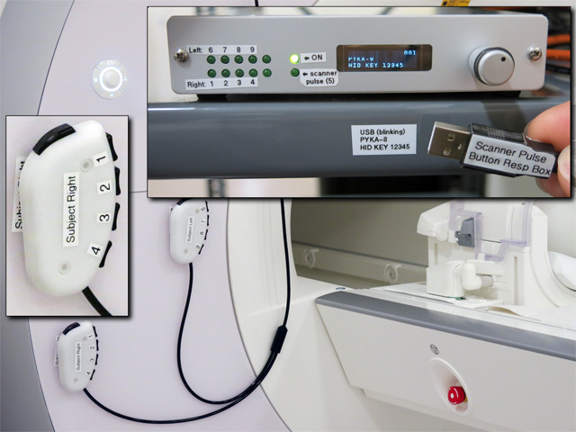
Scanner Pulse and Bimanual Response Boxes, Outside Response Box
The Current Designs USB response box control unit (model 932) generates a USB '5' keypress at the start of each new saved fMRI volume. This can be used to start your stimulus program.
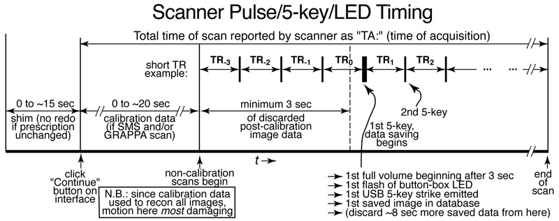
Before saving fMRI data, the scanner may run a shim sequence, as well as several calibration scans (for GRAPPA or SMS), and will then always discard at least 3 seconds of fMRI data before saving (see above). Finally, you will typically want to discard an additional ~8 seconds of the saved imaging data after that (in order for fMRI image brightness to reach a steady state) before starting your stimulus.
N.B.: it is particularly important for subjects to remain still during the calibration scans, since this data is used to reconstruct all subsequent images).
For responses, the Current Designs box generates USB keypresses '1' to '4' (subject right hand, index to little finger), and '6' to '9' (subject left hand, index to little finger). The right and left hand button units are shaped identically, so be sure to pay attention to the labels on them when you set up a subject. The thumb buttons are disabled/fixed. Auto-release is turned ON, so holding down a key will *not* generate a train of characters.
Both the scanner pulse and the subject responses come through a single standard USB cable. When you plug it in, you may initially get a query (e.g., from a Mac) to identify the keyboard type by pressing a particular (non-existent) character. Just ignore the panel ('x' it out), and things will work fine.
After using the button boxes, re-velcro them to the front of the scanner for storage (so they won't drop off the bed and damage the buttons, or get snagged in the table).
There is a single, stand-alone outside-of-the-magnet response box (N.B.: NOT magnet safe!) that can be used for subject practice or for testing response monitoring programs (plugs directly into your laptop like a mouse). It is physically similar to the button boxes in the scanner with two minor differences: (1) the thumb key works, (2) it generates USB keypresses '1' to '5' (thumb to little finger).
Video Connections
The HDMI input cable is on the desk just to the left of the Siemens console computer. There are DVI, display port, and mini-display port adaptors as well as a rescaling analog VGA input convertor box. The native resolution of both projectors is 1920 by 1080 (16x9) and the frame rate is 60 Hz.
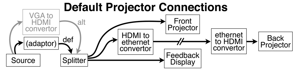
The splitter always sends a signal to the front and rear projectors as well as the console room feedback display.
To turn on the projector, use the "On" button on the remote. When done with a projector, use the smaller blue "Standby" button at the top of the remote to dim the lamp.
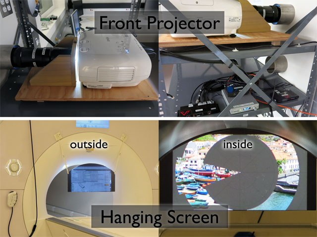
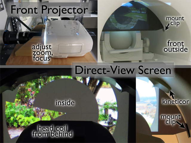
Setting Up the Front Projector (Close-Up/Direct View)
The screen for the front projector is stored on the wall behind the head coils and is hung from two plastic clips on the front of the bore of the magnet after the subject is in the bore. The matte dark gray side should be toward the subject (outside is marked). The rounded upper edges of the screen indicate what is visible to the subject (the circular bore truncates the view of the upper corners of the image).
Slide the mirror on the rails toward almost as far back as possible so subject looks up into the double (uprighting) mirror.
The large, heavy, long-focal-length zoom lens (Navitar MCZ151, 184-314 mm) for the front projector is supported by two triangular wooden struts mounted on a piece of plywood. N.B.: the plywood is attached to a pivot at the front, so don't try to move the front of the base! The Epson 3100 projector sits immediately behind the lens, touching the cork ring, but is not attached to the lens. Don't touch the foot screws on the projector (see below for left/right and up/down adjustments). N.B.: both the zoom and focus accept multiple 360 deg rotations.
If the focus is completely off, a starting point is:
(1) zoom to largest, back off 180 deg smaller
(2) screw focus all the way in to collar, unscrew
180 deg
To adjust image zoom/size, rotate the front part of the lens ("larger" and "smaller" directions are labeled).
To focus the image, rotate the entire lens by grabbing the back part lens closest to the collar (labeled "focus"). This is much more difficult to rotate than the zoom ring.
To adjust the left/right placement of the image, look through the lower wave guide while making small left/right movements of end of the plywood base closest to you (the base will rotate around the front pivot). Moving the end of the plywood to the left moves the image to the right and vice versa (the "up/down" and "left/right" dials on the front of the projector have no effect since the lens is not attached to the projector).
The up/down placement of the image should be OK. If it needs to be adjusted, use the foot screw at the back of the plywood.
A good way to focus is to have an assistant look at the image from behind the magnet before the subject is inside. Then begin to slowly rotate the lens in one direction with both hands, asking the assistant to loudly say "stop" when focus is good. Focus will never be perfect. Then temporarily remove the hanging screen, block the projector beam from inside the room with the cardboard cap, load the subject, replace the screen, and finally unblock the projector.
A 'bug' of the easier-to-turn zoom ring is that it also adjusts focus. This can be a feature. Once zoom and focus are approximately correct, it's actually easier to adjust fine focus with the zoom ring ☺.
Setting Up the Front Projector (Close-Up/Direct View)
The direct-view setup (no mirror) provides the largest visual angle by far, which is useful for retinotopic mapping, immersive stimuli, and studies in extrapersonal space.
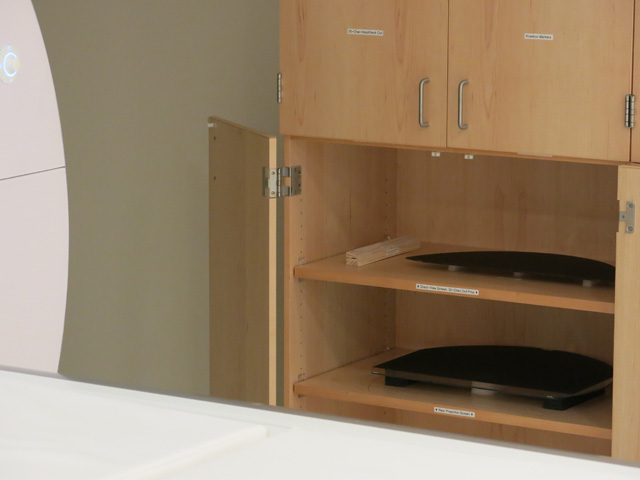
Before putting the subject on the bed, put in the direct-view screen and adjust the zoom/focus/placement of the image. The screen is stored on foam pads in the left wooden cabinet (lower left doors). From the front of the bore, insert the screen with the dull gray side inward (toward the subject). First touch the top of the screen against the Kineticor camera wing, then tuck the left and right bottom edges of the screen into the small clips velcroed to the sides of the bore.
From maximum zoom, back off about 3/4 of a turn. Approximate focus is about 3/4 of a turn from completely screwed in. Finally, adjust the height by raising the leveler screw at the back until the nut is flush with the end of the bolt (this moves the image down on the screen).
Now, remove the bed cushions and the head coil, and put the thin lower back support cushion on the bed. Then insert the wooden head coil prop. Put the head end of the 30-channel head coil on the prop, plug in the top and bottom cables, and finally insert the small wooden cable prop to ensure good contact for the cable coming from the top of the head coil. Tilting the coil and removing the cushions rotates the subject's head forward, making it much easier to directly view the close-up screen. Be sure to provide additional padding for the neck and elbows.
Finally, remember to remove the direct view screen before moving the bed out! (the screen is designed to easily pop off the support clips with a just light touch, just in case).
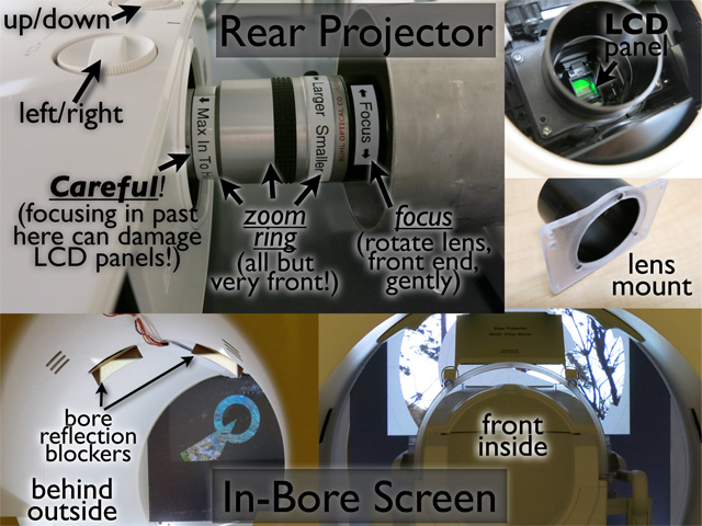
Setting Up the Rear Projector
The rear projector is located in the equipment room. First, go in there and turn it on (with the remote back there) before returning to the control room to plug the video cable into your laptop.
The in-bore screen for the rear projector is stored on foam pads in the left wooden cabinet (lower left doors). From the back of the bore, insert the screen with the dull gray side inward (toward the subject). Tilt the top of the screen inward and insert the top into the small clips just to the right of the Kineticor cable run. Then push the bottom of the screen forward until it hits the two small clips on the light rails.
Use the single rear-projector mirror (for the 30/32 channel coils, the front mirror pair has been removed), or slide the 64-channel mirror (modified rear-projector version under construction) toward the subject's feet so the subject looks up into the single mirror, not the double mirror.
Since the cable run is so long, the HDMI signal has to be converted to use a long ethernet cable running over the magnet room, then converted back to HDMI near the projector. If everything is working right, there should be a green blinking "Status" light on both front and back "HDBaseT" convertor boxes.
Since the rear projector screen is closer, the replacement zoom lens (Navitar MCZ500, 75-125 mm) spans shorter focal lengths, and is smaller. The focus and zoom rings are in opposite positions compared to the front projector lens. Also in contrast to the front projector, the smaller rear projector lens is attached to the projector. The projector should be properly centered and focused. If you decide to move the projector anyway, don't accidentally snap off the lens.
To adjust zoom/size, rotate the labeled zoom ring at the middle of the lens. Peer through the bottom wave guide to see the projected image.
To adjust focus (do this after zooming), gently rotate the labeled ring at the very front of the lens, taking care to support the lens. Be sure that you don't screw the lens too far into the projector (there is a label "Max In to Here"). If you go more than a few mm past that point, you risk having the lens hit and possibly damage the LCD panels.
To adjust the left/right and up/down placement of the image, first roughly center the image by moving the whole projector, taking care to keep the attached lens in the center of the wave guide! Then, rotate the up/down and left/right adjustment dials at the front of the projector for fine adjustments (alternate between making an adjustment, and then peering through the lower wave guide to see the effect).
Projector Image 'Flips' for Front and Rear Projection
There are 4 different possible projector setups:
- rear projector, single mirror (large visual angle)
- front projector, double mirror (upright view, medium visual angle)
- front projector, single mirror (upside down view, slightly larger visual angle)
- front projector, direct-view (in-bore screen, no mirror, largest visual angle)
- "Menu" button
- 3 down arrows (to "Extended" menu item)
- 1 right arrow (pick it)
- 2 down arrows (to "Projection" submenu item)
- Enter (pick it)
- down arrow(s) to select Projection options 1-4
- Enter (to save, survives shutdown)
- "Menu" to close
Here is a table of which setting to pick:
   Menu Item       Mirror Used    Projector Used      Experimenter's View
=============================================================================
1. Front           single         Rear Projector      Normal
2. Front/Ceiling   single         Front Projector     Upside Down
3. Rear            double/none    Front Projector     L/R Flip
4. Rear/Ceiling    ------- [not used] ----------      Upside Down + L/R Flip
=============================================================================
N.B.: There is an extremely confusing mapping between the Front/Rear Menu items, the front/rear projectors, and what the screen looks like from outside the bore ("Experimenter's View" above). The subject, of course, always sees a right-side up, non-left/right-flipped image.
N.B.: The projector-menu items and text may be flipped and/or upside down from outside the bore! So just slavishly follow the recipe of clicks above! If you make a mistake, simply click the "Menu" button again to quit, and start over.
Visual Angle of Image
Visual angle (e.g., of an object on screen) is measured at the eye. Here is a unix command line script to approximate it given image width on the screen and eye-to-screen distance. Measure the eye-to-screen distance w/string and incl. the path before and after any mirror(s):
---------- visual angle script: cut here, chmod ugo+x ------------------------
#! /usr/bin/tclsh
if { [llength $argv] != 2 } { puts "use: visangle <dist> <width>"; exit }
set angle [expr atan2([lindex $argv 0]/2.0,[lindex $argv 1])*180.0/3.1416 * 2.0]
puts "visual angle = [format %2.1f $angle] deg"
--------- visual angle script: cut here --------------------------------------
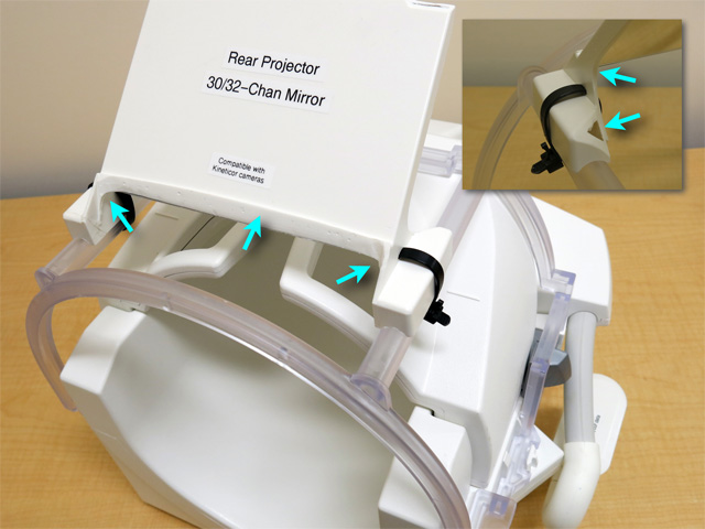
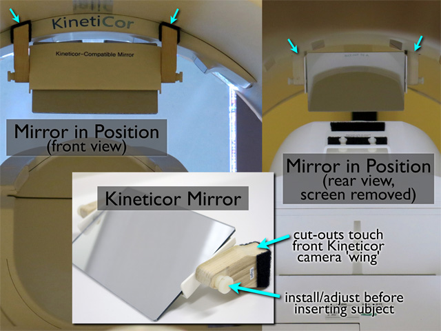
Kineticor-Compatible Mirror
The Kineticor-compatible mirror is stored in the Kineticor cabinet (top left) behind the nose markers. It allows all 4 cameras to see the nose markers. For rear projection, it should be installed and adjusted by the experimenter before inserting the subject (it easily clears the head coil/subject). It is velcroed to the top of the bore with the rounded cut-outs in the wooden supports touching the front of the Kineticor camera 'wing'.
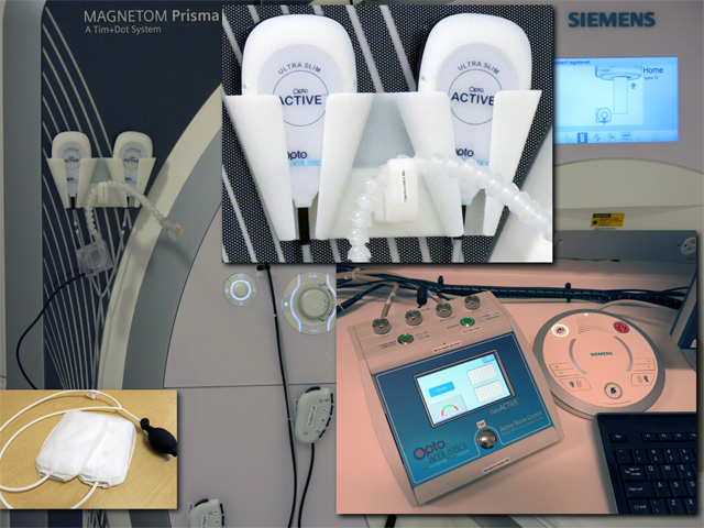
OptoAcoustics Headphones/Mic Operation
The OptoAcoustics noise-cancelling headphones/microphone system is parallel to the Siemens intercom, which still works. You can continue to use the Siemens system if you prefer. The OptoAcoustics system consists of a noise-cancelling microphone, a pair of slim, noise-cancelling earphone units that fit into both 32- and 64-channel coils, and slim inflatable outer pillows that slip in between the headphones and head coil to evenly hold the headphones in place.
The gooseneck microphone (double optical microphone) permits recording completely un-artifacted vocal responses during scans and provides extremely clear subject feedback (disposable pop-filters in cabinet). In contrast to the Siemens intercom, the EPI beeps are completely suppressed, allowing you to even hear the subject whispering during a scan. It's worth telling subjects to speak very softly (also better for position stability). The headphones have piezoelectric drivers and each contains another optical microphone for noise cancellation, but also for recording exactly what the subject is hearing and for setting absolute stimulus sound pressure levels (SPL and spectrum visible on OptoAcoustics console). The OptoAcoustics feedback speaker can be switched between the subject microphone (what the subject is saying -- default: button out) and the internal headphone microphones (what the subject is hearing).
The headphones have clear plastic covers for the black foam ear cushions which should be cleaned with alcohol between subjects rather than immediately discarded. They can be replaced at longer intervals.
Remember that scanner noise gets into your ears via two paths. The first is through the outer ear into the ear canal. The second is via 'bone conduction' directly into the inner ear (vibration of the head in contact with the head coil, sound in the air entering the body and being transmitted to the inner ear). Noise cancelling earphones (and ear plugs) can only cancel (block) noise coming into the ear canal, but not noise entering via 'bone-conduction'. The noise-cancellation performance of the OptoAcoustics system is comparable to well-seated ear plugs. But then they make it possible to deliver high quality auditory stimuli with very easy setup.
The OptoAcoustics system uses an initial 16 sec period (after the first scanner pulse) to 'learn' the spectrum of the repeated noise. During this time, no audio stimulus should be presented. In order to obtain enough samples, the TR (repeated scanner sound) must be less than 3.6 sec. During this initial period, there is no noise cancellation. However, the sealed headphones themselves provide good attentuation of the scanner noise. If you repeat the same scan, you can skip this step, and therefore, reduce the initial 16 sec discarded data period on subsequent scans.
The audio input to the system is via a 3.5mm stereo headphone jack (LINE1) on the back of the OptoAcoustics control unit (in laptop cable bundle on desktop). An optical audio input is also accepted (LINE2, rarely used). The noise-cancelled output of the subject microphone can be recorded along with the scanner trigger pulse via a stereo USB audio connection to the OptoAcoustics control unit. The stereo audio signal heard by the subject (after noise cancellation) can be recorded via the green analog stereo 3.5mm jack on front of the PC-like box under the desk in the corner. The operator mic volume is controlled by an unlabled black knob on the left back of the OptoAcoustics control unit. Finally, there is an alternate operator mic input (3.5mm jack) on the back of the OptoAcoustics control unit (N.B.: plugging something into this jack will disable the built-in operator mic!).
Finally, the subject's microphone signal can be fed back into the headphones to enable more naturalistic speaking (Self-Hearing dial).
Minimal HOWTO:
(1) Turn on OptoAcoustic desktop unit (back panel)
(2) "Start" (touchscreen)
(3) Setup mic/headphones/inflate-pads, move patient table in
(4) "Calibrate" (touchscreen, soft 'whoosh' in each ear)
(5) "Learn" (touchscreen => waits for scanner pulses)
(6) Start scan (noise cancellation starts 16s after 1st scanner pulse)
(7) Start your soundtrack (16s after first scanner pulse)
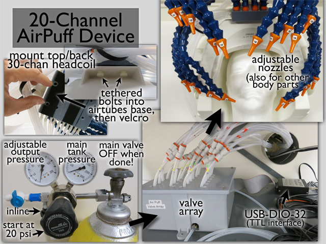
20-channel Somatosensory Air Puffer Operation
The main parts of the system (compressed air cylinder, pressure regulator, valve manifold, air tube bundles, nozzles mounted on Loc-line tubes) are illustrated here. The air tubes are driven by a cylinder of compressed air (medical grade) situated directly to the left of the magnet room door.
The solenoid air valves in this system are controlled by 20 TTL-level lines. Currently, these TTL inputs are connected to a USB-DIO-32 box that converts USB to 32 bits of TTL I/O. There are online Windows and Mac drivers for the USB-DIO-32 system (e.g., to use from MATLAB (mex compiled) or directly from a C program). The Mac version of the mapper program (see below) has support for the USB-DIO-32 USB-to-TTL box.
Finally, the user can directly attach TTL-level signals by disconnecting the female 50 pin ribbon cable from the USB-DIO-32 box (e.g., from a National Instruments digital I/O box), in which case, see the label on the USB-DIO-32 box for pin assignments.
For face stimulation, the array of air tubes can be anchored to the top back end of the 30-channel coil with two tethered nylon bolts, then velcroed. The base of the air tube 'spider' can also be attached to a wooden board with two other nylon bolts for stimulating other body parts.
Minimal HOWTO:(1) turn on and set up TTL valve controller (power switch at low wall socket)
(2) Turn delivered pressure OFF: N.B.: unscrew (CCW) large black knob
(3) Turn main cylinder ON: unscrew (CCW) top valve
(4) Check main cylinder pressure (right gauge) (full cylinder: 2200 psi)
(5) Set 20 psi (left gauge) delivered w/lg black knob (screw in [CW] increases)
(6) open final black in-line valve
When done, reverse procedure. Be sure to verify these two have been done
before leaving:
(A) main air cylinder valve OFF
(B) solenoid valve controller power rocker switch OFF
(at low wall socket)
Logging Siemens Physiological Data (pulse oximeter, respiration)
The CMRR multiband EPI sequence can log timestamped Siemens physiological data events (finger pulse oximeter, breathing belt, ECG, external) and volume acquisition times to text files. To enable this, go to the "System" tab and select the "Special" card (sub-tab). Then select "File" from the "Physio recording" dropdown.
The pulse oximeter is a small bluetooth-connected battery operated device with a finger clip that hangs in a charger cradle in the control room when not in use. The respiration belt is a small air bladder that is strapped around the rib cage. The air tube from the respiration belt plugs into a transducer port in the second battery-operated bluetooth device next to the pulse oximeter. During use, the respiration transducer is placed in a foam holder that rests on the subject's chest.
Before starting the sequence, check if this directory exists:
C:\MedCom\Log\Physio\
If it does, first remove "Physio" and its contents (easiest from Windows
-> Computer; it will be re-created). N.B.: if this directory exists,
the waveforms will still be recorded, but trigger events (see PULS_TRIGGER
annotations below) will not be recorded.
Here is an example of an "Info" file, which contains time timestamped slice and volume acquisition times:
UUID        = 8fcfcebf-41e1-4a1b-b073-6baa0cce69be
ScanDate    = 20210125_114618
LogVersion  = EJA_1
LogDataType = ACQUISITION_INFO
NumSlices   = 48
NumVolumes  = 520
NumEchoes   = 1

VOLUME   SLICE   ACQ_START_TICS  ACQ_FINISH_TICS  ECHO

     0       0         16955546         16955568     0
     0      12         16955546         16955568     0
     0      24         16955546         16955568     0
     0      36         16955546         16955568     0
     0       5         16955579         16955601     0
     0      17         16955579         16955601     0
     0      29         16955579         16955601     0
     0      41         16955579         16955601     0
     ... [rest of the slices for volume 0]
     1       0         16955946         16955968     0
     1      12         16955946         16955968     0
     1      24         16955946         16955968     0
     1      36         16955946         16955968     0
     ... [rest of the volumes]
Here is an example of a "PULS" file, which contains time timestamped pulse oximeter data along with the recognized heatbeat events (that would be used as a trigger):
UUID        = 8fcfcebf-41e1-4a1b-b073-6baa0cce69be
ScanDate    = 20210125_114618
LogVersion  = EJA_1
LogDataType = PULS
SampleTime  = 2

ACQ_TIME_TICS  CHANNEL  VALUE  SIGNAL

     16952318     PULS   3581
     16952320     PULS   3621
     16952322     PULS   3658
     16952324     PULS   3686
     16952326     PULS   3707
     16952328     PULS   3721
     16952330     PULS   3728
     16952332     PULS   3728
     16952334     PULS   3722
     16952336     PULS   3708
     16952338     PULS   3691
     16952340     PULS   3666
     16952342     PULS   3638
     16952344     PULS   3610
     16952346     PULS   3575
     16952348     PULS   3539
     16952350     PULS   3500  PULS_TRIGGER
     16952352     PULS   3460
     16952354     PULS   3418
     16952356     PULS   3376
     16952357     PULS   3334
     ... [rest of the waveform and events]
The log files are appended during the scan. It is the duty of the operator to transfer the temporary files in C:\MedCom\Log\Physio\ to a safe place (e.g., sftp them to the server) immediately after the scan. The filenames are timestamped to the second, so it is safe to put them all in one directory.
By selecting "DICOM" instead of "File", the raw waveform data can instead be saved to a DICOM 'image'. CMRR has matlab code for extracting the waveforms from the pseudo image.
Shimming: Force new shim, Check shim applied, Manual shim
Shimming is a method of re-flattening B0 field after an object has been introduced into the scanner. It works by adjusting continuous currents in the shim coils. The first order shim coils are the X, Y, and Z gradients themselves. Higher order shim coil cause more complex spatial variations in the B0 field (e.g., the Z^2 shim is often used to compensate for the fact that there is a magnetizable body on only one end of the head).
There is a default sets of shim values that work reasonably well for a localizer scan. For most data scans (e.g., MPRAGE, T2* EPI images, EPI diffusion, spectroscopy), the scanner will automatically collect a B0 map and then adjust the shim coil currents based on an analysis of the B0 map. The System -> Adjustments -> B0 Shim mode -> "Standard" acquires only a single B0 map. The "Advanced" mode acquires additional B0 maps and makes successively finer adjustments (takes an additional half a minute).
The volume over which the fieldmap for the shim is collected (the "Adjust" volume) is normally the same as the scan volume, and is indicated by the green box (vs. the yellow box for the scan volume). If you accidentally move or rotate the green shim volume out of alignment with the scan volume, you can restore the default condition of "same as the scan volume" by going to the "System" tab/card on the open protocol, and clicking the "Adjust Volume" sub-tab, and then the "Reset" button.
If a subsequent scan has the same "Adjust" volume (i.e., the volume over which the B0 field has been flattened), the non-default shim values calculated for the previous scan will be used. Sometimes this process can go awry if the EPI phase-encode direction has been changed (e.g., A>>P changed to P>>A) and the scanner software thinks that the "Adjust" volume has therefore been changed. See (2) below for how to fix.
(1) To force a new shim, first load a new scan, then click Options -> Adjust from the right side of the top menu bar (this option will be grayed-out unless a scan has been loaded). This brings up a large "Manual Adjustments" panel. Select "3D Shim" tab (along the bottom), then "Measure" (to acquire a new B0 map), "Calculate" (to determine shim coil currents), and "Apply" (the lower of the two "Apply" button) to use the new shim values for the new scan).
(2) If a subsequent scan is different in any way from the previous one, the shim values for the previous scan may be discarded and the initial global shim defaults (which are set for the localizer) may be used instead. This may or may not trigger an automatic re-shim when you open the new scan. If you open the Options -> Adjust panel and go to "3D Shim" tab as before, you will see two columns of shim coil values, "Temporary" and "System". If you see question marks (?) for the values in the second column, you can use the "Apply" button to copy "Temporary" to "System". The problem is that it is difficult to determine whether the "Temporary" column has been pre-populated with the previous shim values or with the initial global (not very good) shim default values. In general, if you have done a previous manual shim using the Options -> Adjust -> 3D Shim -> Measure/Calculate/Apply method from (1) *and* the new scan is similar or identical, it is safe to use just "Apply" on the new scan (rather than manually running a new shim using the method from (1)).
(3) Finally to (completely) manually shim, select the "Inter. Shim" tab (interactive/manual shim) tab from the bottom of the large Options -> Adjust panel. This starts up a repeated RF pulse (short "tick" once a second) and repeatedly displays the spectrum of the resulting signal (you want it to be narrow and tall). N.B.: Some practice is required to efficiently perform a manual shim with a subject in the magnet! N.B.: A poorly done shim can cause spatial distortion in a B0-sensitive (e.g., BOLD) scan, so unless a subject has moved, it is inadvisable to change the shim in midstream.
The Isocenter
The isocenter is the physical x,y,z center of magnetic field. During typical brain scans, you set the landmark to indicate which head-to-foot point on the subject should be moved to the isocenter when the patient table goes into the magnet. If you collect a default localizer, the point you marked with the laser will be in the center of the localizer images (N.B.: this assumes you didn't reposition the localizer slices themselves before starting the localizer).
If you now set up a second, for example, functional, scan (assuming that you have have System -> Miscellaneous -> Positioning mode set to "REF", our default, which means refer to a reference/localizer scan), you can arbitrarily position your slice block center (and slice block orientation) over the localizer. When you start the scan, the scanner table will NOT move. The block center of the second scan will typically be offset from the magnet isocenter a little bit, but this is no problem, since the magnetic field is quite flat near the isocenter. In general, it's a good thing that the table does NOT move between different scans that have differently positioned slice block centers.
However, if you are scanning a more extended part of the body, you may want the magnet to move the table so that the center of your slice block, wherever you have set it on the localizer, is moved to the isocenter of the magnet. To do this, set System -> Miscellaneous -> Positioning mode set to "ISO" for subsequent scans. Now, when you position a slice block over the localizer and click 'go', the scanner will move the table so that the new scan slice block center ends up at the magnet isocenter. It's good to warn your subject that the table is going to move before you click 'go'. Finally, you may want to position subsequent slice blocks over an extended body part at known relative positions (e.g., to collect slightly overlapping blocks of data). This can be done in a methodical way by making new protocols with non-zero values in the Routine -> Position -> ... -> "H" (head/foot) entry. That number can be positive (toward the head) or negative (toward the foot). For this to work right, the first scan should be collected *without* moving the slice block from its default position.Save/Export/Modify/Import Protocols
There are 3 distinct ways to export a protocol (or protocol group) - as an SQLite database file (*.exar1), an editable ASCII .xml file (*.pro), or as a printable file (*.pdf).
The first format (binary SQLite *.exar1 file) is most useful for backing up a group of protocols or a whole tree of protocols. This can be done by right-clicking on one of the nodes in the protocol tree in the left-hand column when Browsing for protocols in the Dot Cockpit. You can backup different hierarchical levels such as a "program" (a single experiment), an "exam" (a single PI's lab-name), or a "region" (SDSU). This is mainly useful for recovering from console computer hardware failures.
The second format (editable ASCII *.pro file) can be used to save a protocol as an editable XML file. This provides a way to access protocol parameters that may not be exposed in the scanner interface when the protocol is loaded. To export a protocol as a *.pro file, become "Advanced User" (in order to be able to open the "Computer" view of the file system), and then simply drag a protocol out of the Dot Cockpit and drop it into a directory (e.g., U:\tmp). To modify a hidden parameter, carefully edit the *.pro file (using a text editor) and then drag it back into the scan queue to run with modified (hidden) parameters. Finally the protocol (or a protocol group) can be saved as a *.pdf by right clicking on a protocol, a "program" (protocol group), or an "exam" (single PI's lab-name), selecting "Print", then Save as PDF. This method is the most human-readable, but re-import requires hand-typing all the parameters. To print the PDF, save it to U:\tmp, sftp it to the server (commas), make it readable there (chmod ugo+r PDF-file), and open/print it with okular (doesn't dither). (N.B.: trying to print the entire SDSU tree to a PDF may cause a crash).In-house cortical surface mapping software: csurf, mapper
Marty Sereno maintains a software package, 'csurf', for cortical surface-based analysis that can be downloaded for MacOS and Linux operating systems from here:
https://mri.sdsu.edu/sereno/csurf
https://pages.ucsd.edu/~msereno/csurf
This software has user-friendly tools useful for fourier analysis of 'phase-encoded' retinotopic, tonotopic, and somatotopic stimuli. An example stimulus is a flashing wedge periodically rotating around a fixation point, or periodic sweeps in audio frequencies from low to high.
Another software package for generating periodic visual, auditory, and
somatosensory stimuli can be downloaded for MacOS and Linux operating
systems from here:
https://mri.sdsu.edu/sereno/mapper
https://pages.ucsd.edu/~msereno/mapper
These analysis tools can also be used to analyze the spatiotemporal time course of activation in response to any arbitrarily complex, but periodic, task (e.g., reach to eat).
The current csurf distribution includes a new FreeSurfer 'fsaverage' surface
parcellation of cortical areas containing topological maps including
visual, auditory, and somatomotor maps that covers almost 50% of the
neocortex. For more details, see:
Sereno, M.I., M.R. Sood, and R.-S. Huang (2022)
Topological maps and brain computations from low to high.
Frontiers in System Neuroscience 16:787737
(PDF here)
Resources, movies, and atlases
This parcellation provides 117 ROI's for topological maps in each
hemisphere that can be used to analyze any average data that has been
mapped to the FreeSurfer 'fsaverage' surfaces. These ROI's can also be
easily projected back into subject native-space to generate native-space
3D ROI's (see csurf).
This software also contains tools for high-resolution surface reconstruction, that can be used to analyze in vivo scans with higher resolution than the standard 1x1x1 mm scans typically used to make FreeSurfer surfaces. These surfaces will contain a much larger number of vertices (a finer surface mesh) than standard FreesSurfer surfaces.
It is also useful for reconstructing surfaces from very high-resolution post-mortem scans (e.g., cerebellum):
https://mri.sdsu.edu/sereno/cereb
This software is periodically updated (always download latest-dated version). Report bugs in csurf or mapper to msereno at ucsd edu.
How to Power Cycle the Helium Pump
The helium pump should always be on. When it's on, the magnet makes a periodic 'tweet' once a second. After a power cut, even a brief glitch, the helium pump may (very occasionally) not restart properly.
If you are at the magnet when this happens, of if you don't hear this 'magnet heartbeat' return after 5-10 minutes, try power cycling the helium pump in the equipment room (right most cabinet). Here is a video showing how to perform this simple operation:
for Mac OS and Linux. This software is compatible with surfaces generated by the standard FreeSurfer distributions (e.g., freesurfer5.3, freesurfer7.1).